serhii.net
In the middle of the desert you can say anything you want
-
Day 1735 (02 Oct 2023)
Masterarbeit toread stack
Also: 231002-2311 Meta about writing a Masterarbeit
Relevant papers in Zotero will have a ’toread’ tag.
When can we trust model evaluations? — LessWrong
-
How truthful is GPT-3? A benchmark for language models — LessWrong
- paper: [2109.07958] TruthfulQA: Measuring How Models Mimic Human Falsehoods
- especially the bits about constructing and validating!
- sylinrl/TruthfulQA: TruthfulQA: Measuring How Models Imitate Human Falsehoods
- paper: [2109.07958] TruthfulQA: Measuring How Models Mimic Human Falsehoods
-
Code:
- spacy:
- the entire site: Finding linguistic patterns using spaCy
- spacy:
-
lists: AI Evaluations - LessWrong
-
Datasets - The Best Ukrainian Language Datasets of 2022 | Twine some aren’t ones I addedj
-
Victoria Amelina: Ukraine and the meaning of home | Ukraine | The Guardian
-
Ukrainian and Russian: Two Separate Languages and Peoples – Ukrainian Institute of America
-
Bender and friensd:
- Unsupervised Cross-lingual Representation Learning & Unsupervised Cross-lingual Learning - Google Slides
- The cool state and fate paper1 , especially the last bits about language typology.
-
Eval
Python stuff
“Питон для продвинутой группы лингвистов, 2020-2021” (lecture): klyshinsky/AdvancedPyhon_2020_21
I should read through everything here: A quick tour
- HF, LLM etc. Hamel’s Blog - Dataset Basics
-
<_(@inclusion) “The state and fate of linguistic diversity and inclusion in the NLP world” (2020) / Pratik Joshi, Sebastin Santy, Amar Budhiraja, Kalika Bali, Monojit Choudhury: z / https://arxiv.org/abs/2004.09095 / _> ↩︎
Meta about writing a Masterarbeit
Literature review
LessWrong
-
Literature Review For Academic Outsiders: What, How, and Why — LessWrong
-
‘Literature review’ the process is a way to become familiar with what work has already been done in a particular field or subject by searching for and studying previous work
-
Every time I do research I perform a simple thought experiment: assuming somewhere in the world exists evidence that would prove or disprove my hypothesis, where is it?
-
Citations are a hierarchy of ideas
Style etc.
My old note about tenses in a bachelor thesis: Day 155 - serhii.net linking to the excellent Effective Writing | Learn Science at Scitable
- My notes at 231201-1401 How to read and write a paper according to hackernews. Main takeaway for me is to keep in mind my target audience, what they know and what they don’t, when writing.
Grammar glossing
Leipzig glossing rules
Leipzig Glossing rules seems to be the key for me:
-
Markdown and python and stuff
-
Markdown
- cysouw/pandoc-ling: Pandoc Lua filter for linguistic examples
- gunnarnl/pangb4e: Pandoc filter for gb4e support
- parryc/doctor_leipzig: Leipzig, MD - glossing for Markdown
- one can always do
<span style="font-variant:small-caps;">Hello World</span>1
-
Python
-
-
Day 1731 (28 Sep 2023)
Random side quests about the Masterarbeit
UA-RU parallel corpus
pravda.com.ua1 має статті трьома мовами:
- Залужний востаннє поговорив з Міллі на його посаді | Українська правда
- Залужный в последний раз поговорил с Милли в его должности | Украинская правда
- Commander-in-Chief of Ukrainian Armed Forces speaks with Milley for last time before latter steps down | Ukrainska Pravda
The difference seems to be only in that one part of the URL!
Article; title; tags; date,author.
Then article title+classification might be one of the benchmark tasks!
Is there anything stopping me from scraping the hell out of all of it?
Google finds 50k articles in
/eng/, 483k in/rus/, assumption: all english articles were translated to Russian as well.=> For each english article, try to get the Russian and Ukrainian one from the URI.
-
©2000-2023, Українська правда. Використання матеріалів сайту лише за умови посилання (для інтернет-видань - гіперпосилання) на “Українську правду” не нижче третього абзацу.
- Правила використання матеріалів сайтів Інтернет-холдингу ‘‘Українська правда’’ (Оновлено) | Українська правда
Related: ua-datasets/ua_datasets/src/text_classification at main · fido-ai/ua-datasets Related: facebook/flores · Datasets at Hugging Face frow wikinews in infinite languages including UA!
Somehow magically use WikiData
- Douglas Adams - Reasonator
- KGQA/QALD_9_plus: QALD-9-Plus Dataset for Knowledge Graph Question Answering
How does alignment/censoring work with UA?
eg could other langs help for that?2
-
Same goes for Економічна правда and friends. ↩︎
-
(172) Detailed walkthrough of procedure to uncensor models : LocalLLaMA.g. ↩︎
MASTERARBEIT (Master thesis) DRAFT
This will be the Markdown draft of my Master thesis, I’ll jot things down and then expand.
Meta
Canary test
List without newline:
- HTMLsuperscript
- inline $\text{latex}^{\text{superscript}}$
And:
quote without newline
Notation
- Meta
- XXX is for future section numbers and references
- bold is for TODOs and words/formulations I want to replace/rephrase
- TODOs should rather be inside the text than inside footnotes
- Conventions
- Quotes are double-quoted ("") always
- Ukrainian/foreign/historical words (little Russian) are written ось так
- there will/should be no bold in the final thesis text!
- I shall use commas as thousands separator and dots as decimal separator, so US style, not European, because it feels more natural to me and therefore easier to remember.
- Other
- Master’s Thesis, both words capitalized
- Neither “I” nor passive (ChatGPT is good for hard cases)
General
- Add intro text to (sub)sections before starting the sub-sub sections!
Tasks/TODOS/…
- language: make a decision and stick with it everywhere
- (Ukrainian(-language)) NLP (for/in the Ukrainian language)
- “Ukrainian language NLP” and “NLP for the Ukrainian language” are the final contenders.
- bits to check at the end:
- Ctrl-F everything from meta-notation
- URI/URL
- grammar notation
- whether I actually follow my own stated notation rules
- can I remove the complex notation?
- Verbs conjugate, nouns decline, adjectives agree
- bits to remember
- numbers are not numerals!
- Verbs conjugate, nouns decline, adjectives agree
- en-dash, em-dash, etc. 231206-1501 Hyphens vs dashes vs en-dash em-dash minus etc
- CBT: I renamed question/context part to context/challenge segment!
- Conceptual things
- Ctrl-F all the occurrences of “Russian” in the final text and decide on the right balance and nuances, to which extent is it needed
- for every X I use, ask myself the question “why exactly do I use X?”
Links
- 240104-1446 Masterarbeit current status
- 231010-1003 Masterarbeit Tagebuch
- 231203-1745 Masterarbeit eval task LMentry-static-UA
- 231213-1710 Ukrainska Pravda dataset
Benchmark for Evaluation of Language Models in the Ukrainian Language
Thanks and stuff
- X who was the first to made me notice and love language and languages
- all the people who kept this love alive, one way or the other
- CH
- People who have helped proofread or annotate tasks, as well as providing a human baseline:
- M
- KD, KL, -AI etc. etc. etc.
Abbreviations
- ML: Machine Learning
- POS: part of speech
Introduction
Нації вмирають не від інфаркту. Спочатку їм відбирає мову.
Ліна КостенкоNations don’t die from heart attacks. They go mute first.1
(Lina Kostenko, Ukrainian poetess)evals are surprisingly often all you need
(Greg Brockman, OpenAI President)2The Ukrainian language is not at risk of dying, and as of 2023, this much is certain. But before 2014, the quote above was so incisive it hurt.
The last 10 years have led to a resurgence of Ukrainian language, especially its use in informal and non-academic contexts. This was followed by an increase of resources dedicated to its study and use.
On a 2020 survey3 on linguistic diversity in NLP, the Ukrainian language was classed under “rising stars”: languages with a thriving community online but let down by insufficent labeled data.
This Thesis introduces the first Ukrainian-language LM benchmark, and as part of it introduces a number of novel labeled datasets.
- TODOs:
- think about the story I’m telling in the Introduction
- exactly how much Ukrainian history, linguistics and Bender and for what purpose
- In the context of Bender: emphasize how I created datasets
Historical context and bilingualism in the modern Ukrainian language
L’Ukraine a toujours aspiré à être libre
“Ukraine has always aspired to be free.” Voltaire, 1731 4A significant number of people in Ukraine are bilingual (Ukrainian and Russian languages), and most Ukrainians can understand both Russian and Ukrainian 5.
The reasons for this include Ukraine’s geographical and cultural proximity to Russia, as well as of consistent policy first of the Russian empire and the Soviet Union.This section sketches the history of the language, describes the bilingual nature of Ukraine’s society and the impact of historical state policies on its modern development.
(TODO mention how and which tasks are impacted by this; sources for ‘many people believe’; todo tie it with Ukrainians realizing stuff)
- todo: more synonyms for ‘policy’
- todo: better title
- todo: sources for everything-everything-everything
- todo: I don’t need an h4 with one item — move this one level up. Maybe mention Poland, then Russia everything.
- sources
- 1987 book about the entire topic 6
- Article The Executed Renaissance: The Book that Saved Ukrainian Literature from Soviet Oblivion | Article | Culture.pl
- Keeping a record is the best book on this 7
Intro (TODO better title)
The Ukrainian language belongs to the Slavic family of the Indo-European languages (which also contains languages such as Polish, Czech, Serbian, Bulgarian), specifically to the East Slavic branch, which contains Belarusian, Russian, and Ukrainian8. Towards the end of the X century the East Slavonic group of diealects was relatively uniform, with the differences separating Ukrainian, Russian and Belarusian appearing since then, as the result of linguistic and political processes. 9
While all three are mutually intelligible to a certain extent, Ukrainian has more in common with Belarusian than with Russian 9; outside the branch, Ukrainian has partial intelligibility with Polish10.
This stems from the fact that in the 15th century, parts of what is now Ukraine and Belarus were part of the Polish-Lithuanian commonwealth, with Polish becoming the lingua franca of Ukrainian-Belarusian lands.
As a result, a large proportion of the Ukrainian lexicon consists of borrowings from the Polish language, and vocabulary remains the component of the language where the difference with Russian is most immediately noticeable. 9
The suppression of Ukrainian in the Russian Empire
In the Russian Empire, the broader imperial ideology sought to assimilate various ethnicities into a single Russian identity (with Russian as dominant language), and policies aimed at diminshing Ukrainian national self-consciousness were a facet of that.11
Ukrainian (then officially called little Russian 9 and officially a dialect) was12 stigmatized as a strange dialect of Russian, with its literature not taken seriously; the general attitude being that Ukrainians needed to be “civilized” by Russia, by its language and developed culture.11
Attempts to extinguish a separate Ukrainian identity weren’t limited by stigmatization — the history of Ukrainian language bans is long enough to merit a separate Wikipedia page with the list, 13 with the more notable ones in the Russian Empire being the 1863 Valuev Circular (forbidding the use of Ukrainian in religious and educational printed literature)1415 and the Ems Ukaz, a decree by Emperor Alexander II banning the use of the Ukrainian language in print (except for reprinting old documents), forbidding the import of Ukrainian publications and the staging of plays or lectures in Ukrainian (1876)16.
The convergence of Ukrainian and Russian in the Soviet Union
The first decade of Soviet Union brought Ukrainisation as part of a new Soviet nationalities policy, leading to a short-lived period of flourishing for Ukrainian literature and culture in general.17
Many of the Ukrainian writers and intellectuals of that period became later known as “the executed Renaissance”18: most19 of them were purged in the years to follow7, after the Soviet Union took a sharp turn towards Russification in the late 1920s and in the multiple waves of purges afterwards.
Those purged included many of the members of the committee that in 1928 created the first unified Ukrainian spelling rules.20
A new ‘orthographic’ reform was drafted in 1933, without public discussion this time 17. It had the stated goal of removing alleged “burgeoise nationalist” and “pro-Polish” influences in the previous one, especially by the withdrawal of “artificial barriers” between the Ukrainian and Russian languages20. In practice, bringing the Ukrainian language closer to Russian in many ways, from banning the (absent in Russian) letter ґ to introducing changes to grammatical forms 20, adding near absolute reliance on Russian when spelling loanwords and changing the gender of many of them to match Russian, and by making an effort to reduce Ukrainian-specific vocabulary17, especially scientific terminology.
The role of Russian in Soviet society was openly declared to be not just the language of all Soviet peoples, but also the source language for the enrichment of the other languages in the Soviet Union.9
- TODO find some place to fit this:
- One interesting aspect is the asymmetry in language intelligibility: Ukrainians are “clearly more successful” in understanding Russians than vice versa 10. If this mutual understanding was only the result of the closeness of the two languages, there would be no such asymmetry.
Towards the end of the Soviet Era, “it is possible to speak of diglossia in Ukraine, with Russian as the High variety used in formal, administrative, and educational domains, and Ukrainian is less formal, home settings.” 8
After the fall of the Soviet Union, there were many proposals for restoring the original orthography, but only the letter ґ was restored. In 2019 a new version of the Ukrainian orthography was approved, which restored some of the original rules as ’legal’ variants but without mandating any of them.
- TODO sources
The contemporary Ukrainian linguistic landscape
Around 2012, I stumbled upon a forum thread with the topic “I’m moving to Ukraine, which language should I learn, Ukrainian or Russian?”. One answer was “It doesn’t really matter, and if someone will care too much about which language you speak, they are not the people you want to speak to anyway” — not an uncommon sentiment at the time.
For most Ukrainians, the language spoken was/is just not part of one’s self-identification as Ukrainian. Among those surveyed across Ukraine in 2012-2017, only 2.7-4.9% considered the language spoken what determines their nationality (among those who considered themselves Ukrainian it was 1.8-2.5%, Russian — 8.8-15.9%) 5.
It is typical to speak e.g. Russian at school and Ukrainian at home 21, or different languages with different family members (for example, my entire life I spoke Ukrainian with my father and Russian with my mother).
Conversations where different people use Russian or Ukrainian (without any effort awkwardness or negative effects) were (and are) normal as well. This is illustrated by a 2017 survey22 of 2,007 respondents across Ukraine. It found that in the presence of a Ukrainian speaker, 17% of people will speak Russian and ~18% both Russian and Ukrainian (in the other case, ~29% will speak Ukrainian and ~23% both Russian and Ukrainian).
Just as typical is code-switching — changing the language or dialect spoken within the same conversation, sometimes within the same sentence 23. The Parliamentary Code-Switching Corpus paper23 shows examples of this happening for different reasons, such as: inserting quotes/idioms in Russian, using Ukrainian legalese/cliches or law names, switching the language for stylistic purposes (e.g. distinguishing between the official Ukrainian position and a personal one), triggered code-switching (switching the language after using a word or name in the other language), inserting individual words in the other language or just heavily mixing both without clear motivation.
The latter is related to Surzhyk, mixed Russian-Ukrainian speech (variously defined as “a hybrid language that involves Russian and Ukrainian in its creation”24 or “a pejorative collective label for non-standard language varieties”25)[^45], widely spoken (and more rarely written) across Ukraine, especially its eastern, southern and central parts24.
The Russian attack on Crimea in 2014 for many led to stronger attachment to Ukraine and alienation from Russia, with surveys between 2012 and 2017 showing “a consistent and substantial shift”21 from Russian linguistic and ethnic identification towards Ukrainian5, and the full-scale invasion of 2022 accellerated this process, as seen in Rating Group’s March 2022 “Language Issue in Ukraine” survey26.
This was also quantified by an analysis 21 of Ukrainian Twitter data between 13th January 2020 and 10th October 2022, reporting behavioural language changes across Russian-Ukrainian-English while controlling for user turnover (users joining or leaving Twitter).
The plot (adapted from Figure 4 of 21) in Figure XXX shows an increase of the use of Ukrainian over Russian (purple) starting before the full-scale invasion and sharply increasing afterwards.
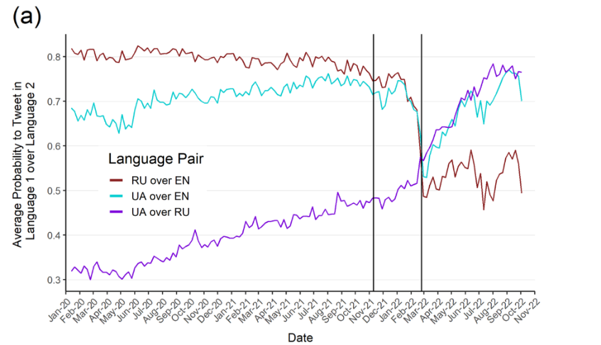
Notably, of the 1,363 users tweeting predominantly (>80%) in Russian before the outbreak of the war, 61% tweeted in Ukrainian more after the outbreak, and ~25% (341) started tweeting predominantly (>80%) in Ukrainian (hard-switch from Russian to Ukrainian). There were only 3% hard-switches from UA to RU in that period.
Ukrainian Twitter users are not a representative sample of the Ukrainian population for several reasons, but the study is likely indicative of wider societal trends.
The authors interpret the switch as users’ conscious choice towards a more Ukrainian identity.27
TODO fit the below somewhere:
- Many Ukrainians started critically reevaluating their language use patterns. (For example, I learned that two friends spoke Ukrainian at home but Russian at school not because they spoke Russian, but because of (basically) peer pressure.)
- mention the diglossia towards the end of USSR
With more people switching to Ukrainian partially or full-time, for different reasons, the importance of Ukrainian NLP grows correspondingly.
Ukrainian as a mid-resource language?
In the taxomy of languages based on data availability 3 (see below), Ukrainian is classified in class 3, “the rising stars”: languages with a thriving online cultural community that got an energy boost from unsupervised pre-training, but let down by insufficient efforts in labeled data collection. Sample languages from that group include Indonesian, Cebuano, Afrikaans, Hebrew. (Russian is in class 4, English and German are in class 5.)
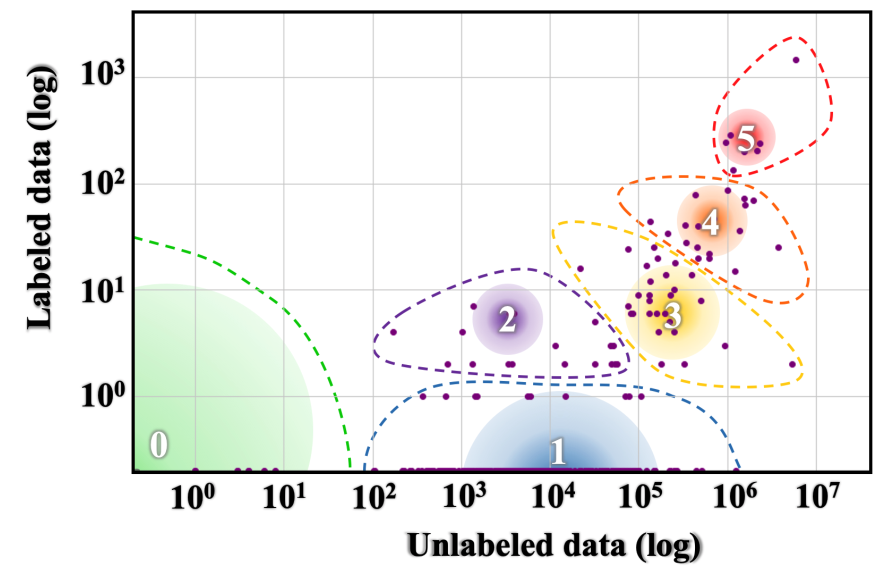 3 as quoted in Why You Should Do NLP Beyond English
From a different angle, looking at estimates of languages used on the Internet (as estimated percentages of the top 10M websites), as of October 2023 Ukrainian is at number 19 (0.6%), between Arabic and Greek2829. English is #1 (53.0%), Russian #3 (4.6%), German at #4 (4.6% as well).
Ukrainian Wikipedia is 15th by daily views and by number of articles30.
The importance of NLP for mid- and low-resource languages
The Bender rule and language independence
Emily M. Bender in 201131 formulated what would come to be known as the Bender rule32: “Name the languages we study”.
Her original 2011 paper — written in the pre-LLM era — discusses the problem of language independence, that is the extent to which NLP research/technology can scale over multiple (or ‘all’) languages. In her more recent writing on the topic, she notes how work on languages other than English is often considered “language specific” and thus viewed as less important 32, and the underlying misconception that English is a sufficiently representative language and therefore work on English is not language specific.
A NLP system that works for English is not guaranteed to behave similarly for other languages, unless explicitly designed and tested for that. Or in different words, “English is Neither Synonymous with Nor Representative of Natural Language”. 32
She highlights 8 proprieties of English that highlight it’s shortcomings in representing all languages, of them 4 apply to Ukrainian: little inflectional morphology, fixed word order, possible matches to database field names or ontology entries, and massive amounts of training data available.
In the context of this thesis, an interesting facet of this issue was my intuitive assumption that Python’s
sort()would sort the letters in their alphabetical order — which is what it does in English — which, for Ukrainian, it didn’t. In hindsight absolutely unsurprising, but I find it absolutely fascinating that for many English-only-speakers many things just work, like python’ssort()doing the intuitively correct thing, and this is taken for granted (along with the assumption that it works for other languages just as well, and that results and approaches generalize). Having for the first time sorted Ukrainian letters in Python I realize how all-encompassing such world models can be. (For details about the sorting issue, see subsection XXX about the LMentry-static-UA task.)(TODO what do I want to say here exactly?)
- Ukr. datasets on the HF Hub being in Russian
- Random list of words contains Russian ones: https://raw.githubusercontent.com/hermitdave/FrequencyWords/master/content/2016/uk/uk_50k.txt
- labs.perplexity.ai models answering in Russian when asked for a Ukrainian folk tale (see Tagebuch for 22-01-2024: 231010-1003 Masterarbeit Tagebuch#^90748a)
Roadmap
This master thesis tackles the following problems in the context of Ukrainian language:
- Research the current state of NLP, especially focusing on the availability and quality of:
- datasets
- corpora
- tools
- literature
- Create novel Ukrainian-language datasets usable as benchmark tasks:
- create human baselines where practicable
- make them publicly available through established platforms
- Create a benchmark for the evaluation of LMs, using both the newly-created datasets/tasks and pre-existing ones
- Evaluate the existing Ukrainian LMs on this benchmark
Additional research questions are:
- Evaluate whether cross/multi language models that include Ukrainian perform equally well to Ukrainian monolingual models
- Research whether there’s a significant difference in scores of tasks translated to Ukrainian using automated methods as opposed to human translations
- Compare the extent to which the language matters when solving problems, with the following languages:
- Ukrainian
- English (high resource language)
- Russian (high resource language from the same language family as Ukrainian)
Theory
Neural networks and stuff
NLP and language modeling
LMs
Transformer-based
LLMs and their magic
LM Evaluation
Intrinsic/extrinsic eval
- Definition and examples
Intrinsic
- Definition
- Examples
- Metrics (Perplexity, bpX etc.)
Extrinsic
- Definition
- Examples
- Metrics
Correlations between them and interplay
Zero/one/few-shot bits
LM benchmarking
Terminology
- from my first paper - task / dataset / benchmark / …
Taxonomy of benchmark tasks
- By task type/goal
- Include more exotic/interesting ones, e.g. truthfulQA33
- One/two/X shot?…
Benchmark data contamination
Canary GUID strings
- My own benchmark tasks have a canary string
- The three ones from ua-datasets don’t, and are too available online - they might have become part of some LLM training data
- Evaluations Canary — Alignment Research Center + BIG benchG
Notable benchmark tasks
- Focus on individual tasks as opposed to bigger things
- The usual ones e.g. in (Super)GLUE
- If other languages’ versions exist - mention them
- Definitely list the ones I’ll use as base
Children’s book test
Other
- TruthfulQA
- Fact completion
Notable benchmarks
- non-UA but multilingual are OK
- general examples and what makes them cool/notable, abstract/high-level, no lists of tasks
HELM!
LMentry
BIGBench
GLUE, SuperGLUE
Benchmark (tasks) desiderata
- How to build a good benchmark (task) in general
- What does
UkrainianNLP need?- Modern but not too modern language
- e.g. not the 1 million word story
- Findability
- Github
- Ease of use
- Upload datasets to HF
- Implementation:
-
Inclusion to other big benchmarks
-
Implementations for important eval harnesses
-
- Modern but not too modern language
Evaluation harnesses
- What and why
- My list in 230928-1735 Other LM Benchmarks notes#’evaluation harness’es
- I decided to use X, instead of writing my own, because
Ukrainian language
Grammatical notation and abbreviations
Glossing notation
Throughout this section, a notation system loosely based on the Leipzig Glossing Rules34 (LGR) for interlinear glossing will be used in examples showcasing Ukrainian language phenomena and translations to English and occasionally German.
Interlinear glosses will not be interlinear, but each gloss will be a superscript to the word it refers to.
For each word, it will be formatted thus:
- The translation will be separated with the grammatical morphemes relating to it by hyphens (-)
- The translation to English will be written in lower case
- The grammatical morphemes will be upper-case abbreviations separated by dots (LGR rule 3).
Not all words of the example will be annotated, only the ones relevant to the example being made. Words already in English will not be translated.
Each translation will be provided on a separate line, with the language marked as ISO 639-3 code:
engfor English,ukrfor Ukrainian,deufor German,rusfor Russian.For example:
eng: the manNOM.SG sawPST the dogNOM.SG
ukr: чоловікman-NOM.SG побачивsaw-PST.MASC.SG собакydog-ACC.SGIn the cases where glosses on morpheme level are needed, the (relevant) segmentable morphemes in the word will be separated by hyphens, and each will have its gloss in its superscript35. The absence of a morpheme needing a corresponding gloss will be marked as $\varnothing$ (LGR Rule 6).
ukr: 5 собакdog-$\varnothing$GEN.PL
Ungrammaticality (examples of grammatically incorrect language) will be denoted by a single asterisk (*) preceding the sentence or the specific word:
ukr: мій *друзь
Abbreviations
These abbreviations are used inside glosses. They are mostly conventional LGR abbreviations36 but contain non-LGR ones as well, given as a separate list.
- Cases
- NOM: Nominative
- ACC: Accusative
- DAT: Dative
- LOC: Locative (’table’ in ’the cup in on the table’)
- VOC: Vocative (used when addressing something)
- Number:
- SG: Singular
- PL: Plural
- 3PL: third person plural (they), 2SG: second person singular (you), etc.
- Gender: M for masculine, F for feminine, N for neutral
- Tenses:
- PST: Past
- FUT: Future
- Other:
- PASS: passive
- REFL: reflexive (deu: ‘sich verspäten’)
- INF: infinitive
- CARD, ORD: cardinal/ordinal numeral
- Verb aspects:
- IPFV: Imperfective (incomplete / habitual actions)
- PFV37: Perfective (completed actions or ones viewed as a single whole).
- Verb moods:
- IMP: Imperative (TODO worth it for confusion with IPFV?)
- Articles:
- DEF, INDEF: definite, indefinite (the/an; der/ein etc.)
- Abbreviations not part of conventional LGR38:
- Parts of speech:
- ADJ: adjective
- PRON: pronoun
- VERB, NOUN: verb, noun
- Morphemes
- PREF: prefix
- STEM: stem
- SUFX: suffix
- Parts of speech:
Ukrainian from a linguistic perspective
Alphabet
- TODO remove this subsection and move the problems paragraph somewhere else.
The Ukrainian alphabet is written in Cyrillic and has 33 letters, in writing the apostrophe and hyphen are also used. It differs from Russian by the absence of the letters ё, ъ, ы and э, and the presence of ґ, є, і, and ї.
This helps (but doesn’t completely solve the problem of) differentiating the two languages, which is needed relatively often: Russian-language fragments within otherwise Ukrainian text (e.g. untranslated quotes in text intended for a bilingual audience) are a typical problem, and one that needs to be solved when building reference corpora or datasets.39
Grammar
Strong morphology
Ukrainian is is a synthetic40 inflected language41, that is it can express different grammatical categories (case, number, gender, ..) as part of word formation. In other words, that information about grammatical categories tends to be encoded inside the words themselves.42
(German, too, is a fusional language, but with a smaller degree of inflection. English, on the other hand, largery abandoned the inflectional case system43 and is an analytic language, conveying grammatical information through word order and prepositions.)
Specifically, Ukrainian:
- nouns decline for the 7 cases44 and 2 numbers (singular, plural)
- adjectives agree with nouns in gender, case, number
- verbs
- conjugate for tenses, voices, persons, numbers
- and in the past tense, they agree with gender as well
- has no articles.
Inflection for word order
The standard word order is Subject-Verb-Object (SVO), but the inflectional paradigm allows free word order. In English the SVO word order in “the man saw the dog” (vs “the dog saw the man”) determines who saw whom. In Ukrainian it’s the last letter of the object (dog) that marks it as such.
eng: the manNOM.SG saw the dogNOM.SG
ukr: чоловікman-NOM.SG побачивsaw собакydog-ACC.SGThis allows the ordering of the words can be used for additional emphases or shades of meaning (similar to German).
A more extensive example:
eng: we foundPST a greenADJ cup NOUN on the table ADJ
ukr: миwe знайшли found-PST.1PL зелену green-ADJ.F.SG.ACC чашку cup-F.SG.ACC наon столі table-M.SG.LOC
deu: wirwe fandenfound-PST.1PL einea-INDEF.F.SG.ACC grünegreen-ADJ.F.SG.ACC Tassecup-F.SG.ACC aufon demthe-DEF.M.SG.DAT Tischtable-M.SG.DATThe amount of categories conveyed by the nouns is roughly similar to German.
Inflection in verbs
Morphology in verbs works in a very similar way. Additionally, unlike other Slavic languages, Ukrainian has an inflectional future tense (formed by a suffix in the verb) in addition to the standard compound future formed by using an auxiliary word бути (“to be”). 45 All this makes longer verbs quite common.
For example, the verb ви́користатиuse-INF.PFV is in perfective aspect, therefore it’s a completed action (“use up” or “utilize completely”) or one seen as a whole even if not completed (“Tomorrow I’ll use my cane to get the pencil from under the bed”)46. It can be transformed into використовуватимутьсяuse-IPFV-FUT-3PL-REFL4748 (3rd person plural imperfect-reflexive-future) thus (in bold the changes):
- використuse-ROOT-аPFV-тиINF: to use (e.g. my cane to get home tomorrow)
- використuse-ROOT-ов-увaIPFV-тиINF: to use (e.g. my cane from time to time)
- використuse-ROOT-ов-увaIPFV-тиINF-мутьFUT.3PL: “They will use their canes”.
- використuse-ROOT-ов-увaIPFV-тиINF-мутьFUT.3PL-сяREFL:
- “The canes will be used tomorrow” (passive)
- “The mice will use themselves to attract the cat into a trap” (reflexive)
Minimal equivalent sentences:
eng: they 3PL willFUT bePASS usedPST.PTCP
deu: siethey werdenwill-FUT.PL verwendetused-PST.PTCP werdenbe-PASS
ukr: вониthey використовуватимутьсяuse-IPFV-FUT-3PL-REFL
rus: ониthey будутbe-FUT.3PL использоватьсяuse-INF-FUT-REFLTodo (This is not a contrived example, використовуватимуться is a natural word in everyday speech.)
- TODO
- do I want this representation? correct it if yes
- A different representation of the Ukrainian sentence:
$\underset{\text{PRON-3PL}}{\overset{\text{they}}{\text{вони}}}$ $\underset{\text{VERB-INF}}{\overset{\text{use}}{\text{використовува-}}}$$\underset{\text{FUT}}{\overset{\text{will}}{\text{ти-}}}$$\underset{\text{VERB-3PL}}{\overset{\text{use}}{\text{му-ть-}}}$$\underset{\text{REFL}}{\overset{\text{themselves}}{\text{ся}}}$
Numerals; agreement of nouns with numerals
Ukrainian numerals can be cardinal (one), ordinal (first) and adverbial (once). They change to varying extent based on case, number49, gender.
The inflection of nouns for (grammatical) number has two classes, singular and plural. Old East Slavic (from which Ukrainian is descended) had a third grammatical number, the dual, since lost50. Some of its traces are in the agreement of nouns and numerals (1 dog, 4 sheep, …).
A simplified51 breakdown follows.
Numerals ending with the following numbers require nouns to:
- 1: agree in gender, number, case with the numeral
- 2, 3, 4: require some nouns to be in the nominative plural, some - nominative singular52
- 5-9, 0, 11-19: require the noun to be in the genitive plural
In practice, this means that “4 dogs” and “5 dogs” have a different plural form for “dog”:
чотириfour-NOM собакdogs-иNOM.PL
пʼятьfive-NOM собакdogs-$\varnothing$GEN.PLThis also means that the numerals (that can be inflected themselves!) have to agree with the noun as well, for example the numeral ‘one’ in ‘one dog’ differs based on case:
ukr: одинone-MASC.NOM.SG собакаdog-MASC.NOM.SG
eng: one dogukr: немаєthere’s no одногоone-GEN.MASC.SG собакиdog-GEN.MASC.SG
eng: one dog is missingLastly, the same holds for larger numerals (“four million”, “five million”) even if they don’t have to agree with any nouns: “million” (thousand, billion, ..) acts as a noun and four/five acts as a numeral, bringing agreement issues even to a stand-alone cardinal number.
-
Todo
- other Numbers to make it clear one is not special
- explain why i can’t replace gen pl with other gen pl - чоловіки and exceptions
-
TODO
-
excellent: http://kulturamovy.univ.kiev.ua/KM/pdfs/Magazine13-16.pdf
-
list: Узгодження числiвникiв з iменниками - Українська мова: від фонетики до морфології
-
complex examples: Узгодження числівника з іменником – Українська мова та література
Implications for NLP
All the above has direct implications for NLP, for example:
- The development of lemmatizers, morphological analyses, bag-of-words approaches for information retrieval31
- In the area of grammatical error correction, systems developed with English in mind perform worse for morphologically rich languages. 53
- Correctly understanding the word order for the tone/intent/emphasis on specific parts of the sentence, as opposed to the arguably more explicit way English conveys this
- Tools written for Russian can be made to work for Ukrainian but this doesn’t happen automatically, because the vocabulary and grammar are different. TODO
- TODO add more and more recent ones
In the context of this Thesis, inflecting words correctly has been the most challenging aspect:
- In the CBT task, replacement nouns had to be inflected correctly so that morphology could not be used to get the correct answer. One initial area of concern was agreement of nouns with numerals — to put the noun in the correct form there could have been a need to track not just the grammatical number (singular/plural), but also the actual number of entities. At the end, this was handled by just using the form of the target word, which had already the correct inflection, and then manually filtering the edge cases. - TODO edit this when I actually do this, I don’t think I’ll have to track enything at the end - gen-pl can replace gen-pl and complex cases can just be excluded from the list
- In the LMentry-static-UA task, different templates that used numbers (“what is the third word in the sentence”, “what is in the third position in the sentence”, etc.) the numbers had to be correctly inflected by case and gender (слово/‘word’ is neutral, позиція/‘position’ is feminine) as well.
- Morphological analyses (needed for later inflection) required disambiguation, since different morphologies or even different POS can be written identically (‘три’ could be a numeral three, or an imperative verb meaning ‘cancel it!’). A correct disambiguation is crucial for future inflection. This necessitated the creation of a separate python package then used by most of the written tasks.
- An additional edge case in the CBT task was that certain words (‘converb’ or ‘adverbial participles’ that share features of both verbs and participles, e.g. приготувавши/готуючи (‘having prepared’ / ‘while preparing’)), tagged by pymorphy2 as POS
GRND( corresponding to the Russian/Ukrainian POS деепричастие54/дієприслівник) are encoded in Universal Dependencies as POSVERBwith featureVerbForm=Conv55 to represent the same concept. And, therefore, are detected as such by spacy’s Morphology. This meant that what spacy detects asVERBs required an additional morphological filtering step to exclude what pymorphy2 would see asGRND, because pymorphy2 isn’t able to inflect between (from its perspective different POS)GRNDandVERB.
For list of other typological features of the language, see its page on the World Atlas of Language Studies5657, as well as the excellent “UD for Ukrainian” page on the Universal Dependencies website58.
Related work
- TODO Everywhere “Ukrainian X” - > “X in the Ukrainian language”??
- The three Ukrainian evals in openai evals! evals/evals/registry/data at main · openai/evals
- GEC!
Ukrainian NLP
State of the research & literature
- Contextual Embeddings for Ukrainian: A Large Language Model Approach to Word Sense Disambiguation - ACL Anthology
- Auto-generating WSD tasks based on SUM dictionary
- The intro of the UA-GEC paper 53 links cool papers about how LMs done with “english in mind” are suboptimal for morphologically rich languages
- robinhad/kruk: Ukrainian instruction-tuned language models and datasets
- and the datasets linked there!
pymorphy2
- Morphology analyzer
- Not perfect for UA.
- no score because no corpus? 59
- Кір. КІР
- also has issues with
цар
- they want to be cited as 60, but I like the arxiv citation a bit more 59
- pymorphy3 exits! not used yet
- does it do probability?..
- faster than spacy
Datasets
- Inclusion criteria: ones that one could conceivably make into a benchmark task
- e.g. not Instructions finetuning
- [2103.16997] UA-GEC: Grammatical Error Correction and Fluency Corpus for the Ukrainian Language53
- Contextual Embeddings for Ukrainian: A Large Language Model Approach to Word Sense Disambiguation - ACL Anthology61
Ukrainian-only
- All
ua-datasets - vkovenko/cross_domain_uk_reviews · Datasets at Hugging Face
Multi/cross/… datasets that include UA
Explicitly mention if it’s google translate or real people did it
-
Belebele Dataset | Papers With Code is a " multiple-choice machine reading comprehension (MRC) dataset", 122 languages
-
KGQA/QALD_9_plus: QALD-9-Plus Dataset for Knowledge Graph Question Answering - one of the 9 langs is Ukrainian! One could theoretically convert the entities into text
-
… somewhere: why can’t one just google translate existing benchmarks and be done with it? precision, eval, etc.
Eval-UA-tion Ukrainian eval benchmark
Basic description
The benchmark contains 2 main tasks:
- CBT-UA (containing XXX test instances), which involves fill-in-the-gaps questions based on children’s stories. Gaps can be of three types: named entities (defined as animate nouns e.g. ‘Whiskers’ or ’tailor’), common nouns (grain, home), and verbs. The goal is that some understanding of the story (characters’ motivations, etc.) is needed to correctly decide e.g. which character was banished from the forest for stealing, or whether he stole grain (owned by his friend) or chickens (owned by his enemy). The idea is based on the Children’s Book Test task 62 but contains many differences from it, most stemming from Ukrainian morphology.
- LMentry-static-UA, which itself is composed of XXX subtasks, some quite different from each other. They are based on tasks that are simple for humans but suprisingly complex for LMs, such as “which word is first in alphabetical order”, “what is the fifth letter of the word ‘orange’”, or “do all words from this list belong to the same category: happiness, sadness, anger, plumber”. It’s based on the LMentry task 63 but departs from it in many ways, form the different subtasks to the change of evaluation mechanism (the original task was scored exclusively by regexes, this task is a dataset with exact anwers, hence the static part in the name).
The tasks and the datasets connected to them are uploaded to the HuggingFace Hub, and EleutherAI lm-evaluation-harness (widely used in literature) ’tasks’ are implemented for each (though not included in the harness itself).
TODO mention how I fulfill the criteria laid out in:
- OpenAI evals checklist
- the multilingual paper bits
- any other similar bits I find
Construction
- CBT task story generation story
Validation and Human evaluation
Validation of the training instances
As a first step, spot-checks of various training instances of the datasets were performed as sanity check.
LMentry-static-UA
LMentry-static-UA contained exclusively algorithmically generated tasks with little randomness involved, and there the validity of the training instances was especially strongly dependent on the code that generated it — and after looking at enough examples of “what’s the Nth word in this sentence”, one could safely assume the rest were likely to be correct as well. So only a limited subset was manually checked.
The only issue found was wrong ground truth in the task about alphabetical ordering: the canonical order of the Ukrainian alphabet is different from what python’s sorting does (with the Ukrainian-only letters і ї є ґ being sorted at the very end instead of their usual place in the Ukrainian alphabet). The relevant code was rewritten to force the correct expected ordering. (Section XXX* has some reflections on the implications of this in the context of the Bender rule.)
CBT-UA
For the CBT-UA task (which involved creating training instances based on data gained through ML approaches), the filtering of the resulting dataset was much more involved.
There were two rough classes of error sources: those caused by language and those caused by logic.
All the failure modes and their numbers are described its subsection XXX, but suffice to say occasional incorrect lemmatization and POS detection by spacy, incorrect normalization and detection (and therefore inflection) by pymorphy2, and the best-guess approach used in the
pymorphy-spacy-disambiguationpackage (written specifically for this Thesis) created a large area of uncertainty.On the logic side, there were the unavoidable errors stemming from the task creation approach (despite reasonable safeguards being put in place where practical), such as multiple possible answers, unknowable answers, etc.
- cases where there was more than one correct answer, e.g.
- if there’s a tailor-turle
- the turtle is a both a turtle and a tailor, and where a gap contained “turtle” using “tailor” there would be correct as well, and both options are included in possible answers:
- “the tailor-turtle started sewing/working”: again, working would be a
Construction, validation, …
- truthfulQA64 paper has examples
- LOOK WHETHER MY BENCHMARK IS PART OF THE TRAINING DATA!!! - doing interesting tests on the topic
Benchmark tasks
POS tagging
UA-SQuAD
LMentry-static-UA
- 231203-1745 Masterarbeit eval task LMentry-static-UA for the progress TODO
This dataset is a set of tasks loosely on the original LMentry evaluation task63 described in section XXX.
- TODO note
- tokenization within sentences (новобранців-іноземців, 100 000)
- within words: пліч-о-пліч how many LETTERS? what about варʼят?
- tokenization within sentences (новобранців-іноземців, 100 000)
Differences from LMentry
The original LMentry 63 had a list of 20-XXX partly repetitive tasks, e.g. “bigger number” and “smaller number” being separate ones.
TODO pic taxonomy of LMentry tasks:

LMentry-static-UA (in addition to applying the ideas to Ukrainian) contains the following conceptual changes:
- Only static tasks are included. The original benchmark uses regular expressions for evaluating the tasks in the included scripts, but regexes are (strictly speaking) needed only for the tasks of type “write word/sentence [(not) containing | starting/ending with ] the following word/letter”. To simplify inclusion in other benchmarks, as well as to not require custom evaluation code, these tasks were dropped, and the LMentry-static-UA tasks can be distributed as-is in the form of datasets.
- Tasks are grouped by type, e.g. task type
CompareTwoThingsis a parent type ofLetterCount(containing both ‘more’ and ’less’ letters) andNumberComparison(bigger+smaller) number. This was done to reduce repetitive code and to decrease the number of tasks to contain only conceptually different ones. - The tasks about first/last entities have been expanded to counting, e.g. in addition to “what is the last word in the sentence” there’s also “what is the fourth letter in this sentence”.
- TODO not yet implemented but will be:
- The task about comparing two numbers has been expanded to basic comparison tasks, e.g. “the red box contains two million pens and the blue box has five hundred thousand thirteen pens; which box has more pens?”
Dataset structure
The LMentry-static-UA dataset is shared on Huggingface under the link XXX. Since the individual tasks are different, multiple configs are contained in the dataset, with e.g. the
NumberComparisonsubtask being available asdataset = load_dataset("shamotskyi/lmentry-static-UA", "numbercomparison")Dataset construction
- Different templates for the same question
- UUIDs to make analysis simpler
- Metadata
List of tasks included
Human evaluation
Challenges in the implementation
Agreement
As with other tasks, agreement of Ukrainian numerals and nouns (see section XXX) has taken a large amount of time.
The different templates contained different nouns in the same role (first word, word one, first position, etc.) that required cardinal and ordinal numerals. They had to agree with the noun in gender (number as well, but in practice only singular was needed TODO):
eng: The third word in the sentence is …
ukr: Третєthird-3SG.N.ORD словоword-3SG.N …This raised two problems.
Encoding and formalization
When creating a template, where/how to encode whether this template requires an ordinal/cardinal and agreed to which grammatical categories.
SOLUTION: including capitalized numerals in the correct form in the template itself and automatically parsing the grammatical categories needed from them:
eng: The FIRSTORD word in the sentence is …
eng: Word number ONECARD in the sentence is …
ukr: ПЕРШЕfirst-3SG.N.ORD словоword-3SG.N …This allowed to create templates using natural language and simplified the data structures involved.
Creation of the training instances with agreemeent
When constructing the actual training instances from the templates:
- all capitalized words are morphologically analyzed with pymorphy2 to get the needed grammatical categories
- the int number needed for the training instance is converted to either ordinal or cardinal numeral in the normal form (
NOM.M.SG) - the resulting numeral in inflected to match the capitalized word in the template
The implementation of this was challenging, and resulted in the creation of a separate pyhon package, ukr_numbers, which creates numerals based on an input integer and a natural language description of the needed inflection:
>>> from ukr_numbers import Numbers
>>> Numbers().convert_to_auto(15,"перший")
'пʼятнадцятий'

# loosely paraphrasing to English:
>>> convert_to_auto(15, "first")
"fifteenth"`
Under the hood, it uses num2words to generate Ukrainian ordinals/cardinals in normal form and the already mentioned pymorphy2 to parse the natural language form and inflect the numeral.
The otherwise excellent
num2wordswas not able to inflect Ukrainian ordinals by case, necessitating manual pymorphy2 inflection logic and leading to many edge cases:- pymorphy2 can analyze and inflect only single words (Ukrainian numerals can contain multiple words)
- disambiguating between different pymorphy2 analyses was complex
- some cases were trivial, e.g. some words being parsed as both verbs and numerals (триthree-NUM / триcancel-2SG.IMP) was not an issue because we know we’re dealing with numerals
- some harder but not an issue, e.g. some grammatical categories can’t be disambiguated from the word itself (e.g. першийfirst-ORD.M?/N? can be masculine or neutral) but this doesn’t matter because after inflection they will be indistinguishable as well
- etc. TODO
- inflecting multiple-word numerals was a whole bundle of joy
- ordinals ending in 10^2 or 10^3, 10^6, 10^9 .. are written together (3000 -> тритисячний), others aren’t (3001-> три тисячі перший)
- in “one/four/five thousand/millions/…”, million acts as a noun, necessitating noun and numeral agreement. And as mentioned in section XXX, nouns take different forms based not on singular/plural, but the actual number involved (plurals aren’t just plurals, 2-3-4 are different from 5+)
- singular/plural conversions for Ukrainian in pymorphy2 was broken, along with the function
make_agree_with_numberthat depended on it, leading to a bug report65 and cumbersome workaround from my side
- singular/plural conversions for Ukrainian in pymorphy2 was broken, along with the function
Not all edge cases are solved, but in all cases relevant to the LMentry-static-UA tasks it works as expected and produces grammatically and semantically correct output.
Children’s book test (CBT)
Basics
TODO The following terms will be used throughout this section:
- A story is divided into two parts, the context segment (the first 65% of the sentences) and the challenge segment (the last 35%).
- The challenge segment contains a gap: the place where a token is masked/removed (replaced with
_____). - The taks is multiple-choice, with options being the 6 tokens provided as possible replacements, only one of them being the correct answer.
- A single test instance (with a gap and corresponding options) is a task instance.
A taxonomy of ways task instances can be wrong
During manual task instance filtering, the task instances were classified into usable and unusable, with the latter removed from the dataset. There were different reasons an instance would be unusable. These reasons were formalized into a simple taxonomy. This was originally done for the people helping with the filtering, in the form of annotation guidelines and with checkboxes in the labeling interface serving chiefly as reminders of the problems to look for.
The errors can be divided into three different (albeit fuzzy) types:
- Logic/continuity errors:
- Cause:
- The way the tasks are created, which doesn’t take into accounts the fact that different words belonging to the classes of the gap may refer to the same entity
- The decision where to place gaps doesn’t take into account the story narrative (but only the location of the gap, frequency of the lemma, and availability of enough different options)
- Kinds:
- Answer unknown - The story doesn’t contain information that allows the answer to be inferred. - > The Cat and the Turtle go to Cat/Turtle/Lion’s house to sew the coat, and later deliver it to the Lion’s house. - The house is mentioned only once and has no dependencies to the rest of the narrative. One can infer that it’s not the Lion’s house (since it’s clearly a different place they have to go to), but there’s no way to know if it was Cat’s or Turtle’s. - However, if the options were only “Cat/Lion’s house” this would be a valid, solvable instance. - Similarly, if the Cat lived in a castle, this would also be considered a solvable instance.
- Multiple options are correct
- It’s clear what entity/action is involved, but there are multiple options which fit it.
-
The Lion liked the Cat and Turtle’s coat/work. Both tailors/animals were happy.
-
Whiskers was happy that he was a cat: he was fast and could climb trees. One morning, he heard his owner say: “Our Whiskers/cat is the fastest cat I know”.
-
- This differs from the previous “answer unknown” case by the fact that there’s no ambiguity about the story itself, only about which word specifically was used.
- It’s clear what entity/action is involved, but there are multiple options which fit it.
- None of the options is correct
- Not found in the filtered instances, would have applied if the correct answer was not found in the options list (e.g. through erroneous removal by the task generation script).
- Duplicate options
- Either two identical options (cat/cat) or slightly differing ones but clearly pointing to the same entity.
- For example, the story has a small bird, occasionally referred to as birdie, both words get lemmatized into two different lemmas, don’t get deduplicated, and both appear as options.
- In Ukrainian, reflexive verbs ending in “-ся” (-sja) before certain consonants can have the ending shortened into “-сь” (-s’), while remaining the exact same verb
- Note that if there are two different characters, e.g. the large Bird and the small Birdie, then these words would refer to different characters and this error won’t apply.
- Differs from “multiple options are correct” by the fact that here it’s not different facets of the same entity (sewing is a type of work), but they are exactly the same entity.
- Cause:
- Language errors
- Cause:
- incorrect filtering of nouns by gender
- non-existing words introduced to the story itself during generation
- incorrect morphology parsing, lemmatization/normalization, inflection, and errors in the related code
- Types:
- Ungrammatical words in options
- Sometimes, the parsing-normalization-inflection pipeline failed in ways that led to words inflected with wrong rules, creating invalid words
- For example, другfriend-SG’s plural is друзіfriends-PL. This plural form, when inflected back into singular with pymorphy, resulted in the ungrammatical *друзьSG. The logic behind this transformation fits some existing inflection paradigms of the Ukrainian language: for example, nouns of Declension III66 ending with “-ь” in singular do end with “-і” (тінь-тіні, область-області) in plural. But друг is a Declension II noun, and features a root consonant alternation г->з. In other words, the plural of the Declension II noun gets transformed into singular using Declension III rules, ending up with a whole new ‘word’. This is especially notable because of just how common the word “friend” is.
- Another source of strange words were the stories themselves. GPT4 (TODO: exact model) especially had difficulties with genders in general, and sometimes attempted to create feminine versions of masculine-only nouns, one notable example being метелицяsnowstorm-F — used as an (incorrect) feminine version of метеликbutterfly-M, which is a masculine noun that has no corresponding feminine. (If it had, метелиця might have been it, since this is exactly how feminine words are often formed: працівник/працівниця.) Most such cases were removed during the story editing process.
- Sometimes, the parsing-normalization-inflection pipeline failed in ways that led to words inflected with wrong rules, creating invalid words
- Option in the wrong inflection
- The process that selects and inflects options to the same inflection as the correct answer failed, creating a grammatically correct word that would create an ungrammatical sentence if put in the gap, thereby leaking information.
-
She yelled/speaking at both dogs/cats/butterfly.
- After ‘both’ clearly a plural is expected, the option ‘butterfly’ is singular and therefore not the correct answer; similarly, the needed verb is definitely not an infinitive.
-
- Given the inflectional nature of Ukrainian, the number of different variations of this error were immense.
- Exceptions to this rule were:
- The “most frequent (all genders) distractor”, if present, was allowed to be of a different gender.
- Verbs were inflected by aspect/tense/number/gender/person but this was rarely enough to hide grammatical information, and can be excluded especially by transitivity/intransitivity. This is a known issue and not considered an error in this context.
- The process that selects and inflects options to the same inflection as the correct answer failed, creating a grammatically correct word that would create an ungrammatical sentence if put in the gap, thereby leaking information.
- Ungrammatical words in options
- Cause:
- Other errors:
- Grammatical errors in the story text itself
- Others
Some of these issues were dealt with fixes/rewrites the code, e.g.:
- rewriting some spacy’s lemmas (in the cases where the systematical errors were in frequent nouns; interestingly most such errors seemed to be caused by Russian influence), among the fixed ones were:
- Миша, Люди (eng: Mouse, People) were parsed as (respectively) the Russian diminutive of the name Михаил/Michael and as the Ukrainian possessive from the diminutive of the name Людмила/Ludmila.
- котаcat-SG.ACC67 was lemmatized as кот, a word which doesn’t exist in Ukrainian but is the correct Russian normal form of ‘cat’ (the correct Ukrainian normal form would have been кіт).
- See Appendix XXX for the full list of rewrites used during task generation.
- simply replacing problematic words in text:
- *заяць was replaced with заєцьrabbit: GPT4 consistently used the wrong word for rabbit, and was quite emphatic about it being the only correct form when challenged — it isn’t, this word doesn’t exist in Ukrainian except as last name, and the “я” in the root clearly comes from the Russian word for rabbit, заяц.
- blacklisting some common problematic words which were not worth the effort to fix, as well as frequent verbs which weren’t good candidates for either gaps or options.
TODOs
-
Original English thing62
-
My current task notes page is 231024-1704 Master thesis task CBT
-
Get Ukrainian book with good OCR, POS-tag, generate questions, manually check
-
Mention how it’s more interesting in Ukrainian than English because morphology - need to do agreements etc.
-
paper:
- they don’t anonymise stuff because 2015 and background knowledge is good - we do the opposite
- it’s really large
- they do baselines, e.g. most frequent word etc.!
- human eval
- once only question, once question+context
- w/o context, models are better than humans?
- language styles
- they didn’t filter the questions, but used humans as baseline to measure performance on the task — this means that I can too do the same?!
-
Similar: demelin/understanding_fables · Datasets at Hugging Face
-
Corner cases:
- Черепаха і черепашка edge case
- Рада слонів — Gemini likes being more creative
- король лев / подякувала королю-леву
- sometimes generated it in Russian
- зайчик/заєць and distractors that already exist
- не називав черепаху лінивОЮ — no way to get around the linguistical information
- anmials named Швидкий/Грізний that work with disambiguation if pymorphy gives this option, but it doesn’t always
- multiple options correct: черепаха/кравчиня віднесла костюм леву (note that both are animate!j)
-
Safety
Вовк і лисиця підстерегли черепаху в лісі і напали на неї. Черепаха не могла втекти і захиститися і стала благати про пощаду. Але вовк і лисиця були безжальні і розірвали черепаху на шматки.
(Pdb++) response.prompt_feedback block_reason: SAFETY safety_ratings { category: HARM_CATEGORY_SEXUALLY_EXPLICIT probability: NEGLIGIBLE } safety_ratings { category: HARM_CATEGORY_HATE_SPEECH probability: NEGLIGIBLE } safety_ratings { category: HARM_CATEGORY_HARASSMENT probability: MEDIUM } safety_ratings { category: HARM_CATEGORY_DANGEROUS_CONTENT probability: NEGLIGIBLE }-
Fixing gpt4 stories with gemini works!
-
Леопард, відчуваючи респект, кивнув у знак схвалення, і Жук також не міг приховати свого здивування тонкістю роботи.
-
Леопард, відчуваючи повагу, кивнув у знак схвалення, а Жук не міг приховати свого здивування тонкістю роботи.
-
Gemini is better at other languages: neulab/gemini-benchmark
Stories criteria
- Too many clear gender errors (main character has wrong gender from the start)
- Complex cases like Рада слонів or things like “the two kittens”
- Clearly nonsensical
- Too short or too few characters
Russian-Ukrainian interference test
- Auto-complete sentences based on:
Modern Ukrainian language + genders
- Check whether the model correctly uses the newer grammar, especially including захисниЦЯ etc. (but not war-related words) 68 by letting it autocomplete things
Ukrainska Pravda news article classification
SECTION LOCATED HERE: 231213-1710 Ukrainska Pravda dataset
Validation
- Ask X people to solve the entire (or a subset) of the tasks, see how many they get right
- Prolly google spreadsheet
Experiments
Models tested on the new benchmark
-
for ideas about it, see truthfulQA paper33 as well as any multi-lingual benchmark paper
-
openAI API
-
On LM harness scores for multiple choice acc VS
acc_norm -
Instructions
- (as required by many models, e.g. Radu1999/Mistral-Instruct-Ukrainian-SFT · Hugging Face)
- Templates for Chat Models
Downstream task: News classification (NC)
Experiments
Do UP news classification with different models, do pretty graph about how it correlates with my benchmark results.
Conclusion
Appendixes
Appendixes A: regexes for skipping paragraphs in UPravda dataset
!231213-1710 Ukrainska Pravda dataset#Appendixes A regexes for skipping paragraphs in UPravda dataset
Appendix B: rewrites and distractors used during CBT task instances generation
This config file contains both lemma fixes, word replacements and word blacklists as well as the distractors used during CBT instance geneation.
lemma_fixes:
    миш: миша  # people named Михайло
    люди: люди  # people named Люда
    люда: люди
    кота: кіт  # not кот
    кот: кіт  # not кот

    # а не вбивець
    # EDIT ACTUALLY it exists, though infrequently https://goroh.pp.ua/%D0%A7%D0%B0%D1%81%D1%82%D0%BE%D1%82%D0%B0/%D1%83%D0%B1%D0%B8%D0%B2%D0%B5%D1%86%D1%8C
    # pymorphy2 and spacy both use вбивець
    вбивці: вбивця

word_replacements:
    заяць: заєць

word_blacklist:
    - шати
    # - мати
    - бути
    - стати
    - могти

distractors:
    NAMED_ENTITY:
        animal:
            male:
                # - собака
                # - кіт
                - їжак
                # - птах
                # - метелик
                - ведмідь
                - півень
                - жираф
                # - дракон
                - слон
                # - ворона
            female:
                - коза
                - жаба
                # - кішка
                - свиня
                - мавпа
                - зозуля
            neutral:
                # TODO add more
                - котеня
                - слоненя
                - зайченя
                - жабеня
                - козеня
                - мавпеня
                - тигреня
                - козеня
                - вовчисько
        human:
            male:
                # - чоловік
                - син
                - багатир
                - Петро
                - лісник
                - селянин
                - чорт
                - домовик
                # - брат
            neutral:
                - дівча
                - дитя
                - немовля
            female:
                - селянка
                - відьма
                - жінка
                - дочка
                - сестра
                - мати
                - королева
    COMMON_NOUN:
        male:
            - автомобіль
            - будинок
            - шлях
            - ящик
            - меч
            - замок
            - стіл
        neutral:
            - дерево
            - яйце
            - ім'я
            - яблуко
            - місто
            - озеро
            - поле
            - вікно
            - ліжко
            - листя
            - шиття
            - мистецтво
        female:
            - гривня
            - природа
            - трава
            - річка
            - книга
            - дорога
            - кімната
-
‘Go mute first’ variation taken from here: Translations ↩︎
-
Greg Brockman on X: “evals are surprisingly often all you need” / X ↩︎
-
<_(@inclusion) “The state and fate of linguistic diversity and inclusion in the NLP world” (2020) / Pratik Joshi, Sebastin Santy, Amar Budhiraja, Kalika Bali, Monojit Choudhury: z / / _> ↩︎ ↩︎ ↩︎
-
TODO format citation Debunking the myth of a divided Ukraine - Atlantic Council citing Oeuvres complètes de Voltaire - Voltaire - Google Books ↩︎
-
<_(@kulyk2018shedding) “Shedding Russianness, recasting Ukrainianness: The post-Euromaidan dynamics of ethnonational identifications in Ukraine” (2018) / Volodymyr Kulyk: z / / _> ↩︎ ↩︎ ↩︎
-
<_(@krawchenko1987social) “Social change and national consciousness in twentieth-century Ukraine” (1987) / Bohdan Krawchenko: z / / _> ↩︎
-
<_(@1130282272476965120) “Keeping a record : Literary purges in Soviet Ukraine (1930s), a bio-bibliography” (1987) / George Stephen Nestor Luckyj: z / https://cir.nii.ac.jp/crid/1130282272476965120 / _> ↩︎ ↩︎ ↩︎
-
<_(@grenoble2010contact) “Contact and the development of the Slavic languages” (2010) / Lenore A Grenoble: z / / _> ↩︎ ↩︎
-
<_(@press2015ukrainian) “Ukrainian: A comprehensive grammar” (2015) / Ian Press, Stefan Pugh: z / / _> ↩︎ ↩︎ ↩︎ ↩︎ ↩︎
-
<_(@rehbein2014check) “How to check understanding across languages. An introduction into the Pragmatic Index of Language Distance (PILaD) usable to measure mutual understanding in receptive multilingualism, illustrated by conversations in Russian, Ukrainian and Polish” (2014) / Jochen Rehbein, Olena Romaniuk: z / / _> ↩︎ ↩︎
-
<_(@doi:10.1016/j.euras.2014.05.005) “Ukraine and russia: Legacies of the imperial past and competing memories” (2014) / Andreas Kappeler: z / https://doi.org/10.1016/j.euras.2014.05.005 / 10.1016/j.euras.2014.05.005 _> ↩︎ ↩︎ ↩︎
-
the primary source11 states that, to a certain extent, among many Russians and some Europeans — still is. ↩︎
-
Also memorably stating that “a separate Little Russian language has never existed, does not exist and cannot exist, and that their dialect, used by commoners, is just the Russian Language, only corrupted by the influence of Poland”72 ↩︎
-
<_(@dibrova2017valuev) “The valuev circular and the end of little russian literature” (2017) / Volodymyr Dibrova: z / / _> ↩︎
-
<_(@remy2017despite) “Despite the valuev directive: Books permitted by the censors in violation of the restrictions against ukrainian publishing, 1864-1904” (2017) / Johannes Remy, others: z / / _> ↩︎
-
<_(@5c48fce9-c05d-3d4e-94c1-cd6079bff660) “The language question in the ukraine in the twentieth century (1900-1941)” (1987) / GEORGE Y. SHEVELOV: z / http://www.jstor.org/stable/41036243 / _> ↩︎ ↩︎ ↩︎
-
<_(@1ad9e7d5-c0eb-33df-ae6c-1fdbd2549d75) “The executed renaissance paradigm revisited” (2004) / HALYNA HRYN: z / http://www.jstor.org/stable/41036862 / _> ↩︎
-
“Of those [lost to Ukrainian literature] 236 were writers. (…) 1,087 writers were active in Ukraine, the loss amounted to 33 per cent.. In terms of figures alone the losses were quite significant, but in terms of literary quality and originality they were devastating.” 7 ↩︎
-
<_(@karunyk2017ukrainian) “The ukrainian spelling reforms, half-reforms, non-reforms and anti-reforms as manifestation of the soviet language policy” (2017) / Kateryna Karunyk: z / / _> ↩︎ ↩︎ ↩︎
-
<_(@Racek2024) “The Russian war in Ukraine increased Ukrainian language use on social media” (2024) / Daniel Racek, Brittany I. Davidson, Paul W. Thurner, Xiao Xiang Zhu, Göran Kauermann: z / https://www.nature.com/articles/s44271-023-00045-6 / 10.1038/s44271-023-00045-6 _> ↩︎ ↩︎ ↩︎ ↩︎
-
<_(@Matveyeva2017) “Modern language situation (on the basis of the 2017 survey)” (2017) / Nataliya Matveyeva: z / http://lcmp.ukma.edu.ua/article/view/123368 / 10.18523/lcmp2522-92812017123368 _> ↩︎
-
<_(@Kanishcheva2023) “The Parliamentary Code-Switching Corpus: Bilingualism in the Ukrainian Parliament in the 1990s-2020s” (2023) / Olha Kanishcheva, Tetiana Kovalova, Maria Shvedova, Ruprecht Von Waldenfels: z / https://aclanthology.org/2023.unlp-1.10 / 10.18653/v1/2023.unlp-1.10 _> ↩︎ ↩︎
-
<_(@Sira2019) “Towards an automatic recognition of mixed languages: The Ukrainian-Russian hybrid language Surzhyk” (2019) / Nataliya Sira, Giorgio Maria Di Nunzio, Viviana Nosilia: z / http://arxiv.org/abs/1912.08582 / _> ↩︎ ↩︎
-
<_(@bernsand2001surzhyk) “Surzhyk and national identity in Ukrainian nationalist language ideology” (2001) / Niklas Bernsand: z / / _> %% %%[^45]: Some 70 even hypothesize two subtypes of it: an older one, created during the times of Russian language dominance when Ukrainian speakers had to adapt, and a newer post-1990 one, born when Russian speakers had to at least partially turn to Ukrainian. ↩︎
-
<_(@ratinggroupSixthNational) “The sixth national poll: The language issue in Ukraine (March 19th, 2022) — Ratinggroup.Ua” (2022) / : z / https://ratinggroup.ua/en/research/ukraine/language_issue_in_ukraine_march_19th_2022.html / _> ↩︎
-
Switching from Russian to Ukrainian, for a Russian speaker, is hard, including emotionally. Mother Tongue: The Story of a Ukrainian Language Convert - New Lines Magazine71 is one of the best articles I’ve read in 2023 and is an excellent description of the topic. ↩︎
-
<_(@enwiki:1182341232) “Languages used on the internet — Wikipedia, the free encyclopedia” (2023) / Wikipedia contributors: z / https://en.wikipedia.org/w/index.php?title=Languages_used_on_the_Internet&oldid=1182341232 / _> ↩︎
-
quoting Usage Statistics and Market Share of Content Languages for Websites, September 2023 ↩︎
-
<_(@wiki:xxx) “List of Wikipedias/Table2 — Meta, discussion about wikimedia projects” (2022) / Meta: z / https://meta.wikimedia.org/w/index.php?title=List_of_Wikipedias/Table2&oldid=23936182 / _> ↩︎
-
<_(@bender) “On achieving and evaluating language-independence in NLP” (2011) / Emily M Bender: z / / _> ↩︎ ↩︎
-
<_(@benderpost) “The #BenderRule: On naming the languages we study and why it matters” (2019) / Emily Bender: z / https://thegradient.pub/the-benderrule-on-naming-the-languages-we-study-and-why-it-matters/ / _> ↩︎ ↩︎ ↩︎
-
TruthfulQA/TruthfulQA.csv at main · sylinrl/TruthfulQA ↩︎ ↩︎
-
<_(@comrie2008leipzig) “The Leipzig Glossing Rules: Conventions for interlinear morpheme-by-morpheme glosses” (2008) / Bernard Comrie, Martin Haspelmath, Balthasar Bickel: z / / _> ↩︎
-
Unless a segmentation is needed only to have an adjacent morpheme that does need a gloss segmented correctly — then such a morpheme may not have a gloss. ↩︎
-
See List of glossing abbreviations - Wikipedia for a full list. ↩︎
-
Not to be confused with PERF (perfect tense), not used in this Thesis. ↩︎
-
Sometimes used, but absent from LGR proper since they are not glosses for morphological values.
↩︎Authors also use placeholders for generic elements in schematicized parsing, such as may be used to illustrate morpheme or word order in a language. Examples include head or hd ‘head’; root or rt ‘root’; stem or st ‘stem’; pref, prfx or px ‘prefix’; suff, sufx or sx ‘suffix’; clit, cl or encl ‘(en)clitic’; prep ‘preposition’ and pos or post ‘postposition’, png ‘person–number–gender element’ and tam ’tense–aspect–mood element’ (also ng number–gender, pn person–number, ta tense–aspect, tame tense–aspect–mood–evidential) etc. These are not listed below as they are not glosses for morphological values. (List of glossing abbreviations - Wikipedia) TODO remove this
-
<_(@9648705) “Ukrainian text preprocessing in GRAC” (2021) / Vasyl Starko, Andriy Rysin, Maria Shvedova: z / / 10.1109/CSIT52700.2021.9648705 _> ↩︎
-
as opposed to analytic languages; Wikipedia has cool bits in Synthetic language - Wikipedia e.g. antidisestablishmentarianism ↩︎
-
also known as fusional language:Fusional language - Wikipedia ↩︎
-
Another way to say this is that synthetic languages are characterized by a higher morpheme-to-word ratio. ↩︎
-
except for personal pronouns; English grammar - Wikipedia ↩︎
-
including the vocative case, absent in Russian, used when adressing someone (e.g. собакdog-аNOM when addressed becomes собакdog-oVOC) ↩︎
-
As an added layer of complexity, word stress can also impact grammatical categories. - TODO emphasize if I actually do a homonym-like task ↩︎
-
nice explanation: TODO removePerfective aspect - Wikipedia / Imperfective aspect - Wikipedia ↩︎
-
Or
Aspect=Imp|Mood=Ind|Number=Plur|Person=3|Tense=Fut|VerbForm=Finin CoNLL-U FEATS format. ↩︎ -
TODO thank him for this word? Daniel Broomfield 🇺🇦🇬🇧 on X: “Найскладніші слова в українській мові для мене: використовуватимуться високопоставленими абищиця (Ніколи не пам’ятаю, де поставити наголос 😑)” / X ↩︎
-
Some nouns can be used only in plural, e.g. in одні окуляри (one pair of glasses) the numeral one is plural! ↩︎
-
Parts of it — to history, other parts — explicitly forbidden in the 1932 grammar reform. ↩︎
-
This is only a partial description of both nouns agreement and numerals declination. ↩︎
-
Mostly for some nouns of male gender (два громадянина) ↩︎
-
<_(@Syvokon2022) “UA-GEC: Grammatical Error Correction and Fluency Corpus for the Ukrainian Language” (2022) / Oleksiy Syvokon, Olena Nahorna: z / / _> ↩︎ ↩︎ ↩︎
-
Обозначения для граммем (русский язык) — Морфологический анализатор pymorphy2 ↩︎
-
<_(@wals) “WALS Online (V2020.3)” (2013) / : z / / 10.5281/zenodo.7385533 _> ↩︎
-
<_(@Korobov2015) “Morphological Analyzer and Generator for Russian and Ukrainian Languages” (2015) / Mikhail Korobov: z / http://arxiv.org/abs/1503.07283 / _> ↩︎ ↩︎
-
<_(@Korobov) “Morphological analyzer and generator for russian and ukrainian languages” () / Mikhail Korobov: z / http://dx.doi.org/10.1007/978-3-319-26123-2_31 / 10.1007/978-3-319-26123-2_31 _> ↩︎
-
<_(@labaContextualEmbeddingsUkrainian2023) “Contextual Embeddings for Ukrainian: A Large Language Model Approach to Word Sense Disambiguation” (2023) / Yurii Laba, Volodymyr Mudryi, Dmytro Chaplynskyi, Mariana Romanyshyn, Oles Dobosevych: z / https://aclanthology.org/2023.unlp-1.2 / 10.18653/v1/2023.unlp-1.2 _> ↩︎
-
<_(@taskCBT) “The goldilocks principle: Reading children’s books with explicit memory representations” (2015) / Felix Hill, Antoine Bordes, Sumit Chopra, Jason Weston: z / / 10.48550/ARXIV.1511.02301 _> ↩︎ ↩︎
-
<_(@bm_lmentry) “LMentry: A language model benchmark of elementary language tasks” (2022) / Avia Efrat, Or Honovich, Omer Levy: z / https://arxiv.org/abs/2211.02069 / 10.48550/ARXIV.2211.02069 _> ↩︎ ↩︎ ↩︎
-
<_(@linTruthfulQAMeasuringHow2022) “TruthfulQA: Measuring How Models Mimic Human Falsehoods” (2022) / Stephanie Lin, Jacob Hilton, Owain Evans: z / / _> ↩︎
-
Числа и проблемы с склонением в разборах всех украинских слов · Issue #169 · pymorphy2/pymorphy2 ↩︎
-
<_(@danylyuk2022main) “The main features of the ukrainian grammar” (2022) / Nina Danylyuk, Tetiana Masytska, Douglas O’Brien, Oksana Rohach: z / / _> ↩︎
-
Strictly speaking, кота can be either ACC or GEN case. ↩︎
-
<_(@synchak2023feminine) “Feminine personal nouns in ukrainian: Dynamics in a corpus” (2023) / Vasyl Starkoand Olena Synchak: z / / _> ↩︎
-
https://chat.openai.com/share/c694b707-4f23-4e57-8ee8-1e560dd3febe ↩︎
-
<_(@hentschel2020ukrainisch) “Ukrainisch-russisches und russisch-ukrainisches Code-Mixing. Untersuchungen in drei Regionen im Süden der Ukraine” (2020) / Gerd Hentschel, Tilmann Reuther: z / / _> ↩︎
-
<_(@newlinesmagMotherTongue) “Mother Tongue: The Story of a Ukrainian Language Convert — Newlinesmag.Com” (2023) / : z / https://newlinesmag.com/first-person/mother-tongue-the-story-of-a-ukrainian-language-convert/ / _> ↩︎
-
<_(@enwikisource:13111073) “Translation:Valuyev circular — Wikisource,” (2023) / Wikisource: z / https://en.wikisource.org/w/index.php?title=Translation:Valuyev_Circular&oldid=13111073 / _> ↩︎
LM Benchmarks notes
Context: 230928-1527 Evaluation benchmark for DE-UA text Here I’ll keep random interesting benchmarks I find.
HELM
- Code
- Random code sample from all common-sense scenarios: helm/src/helm/benchmark/scenarios/commonsense_scenario.py at main · stanford-crfm/helm
- Scenarios: Holistic Evaluation of Language Models (HELM)
GLUECoS
code: GLUECoS/Code at master · microsoft/GLUECoS
Cross-lingual
XGLUE
- microsoft/XGLUE: Cross-lingual GLUE
- Interesting enough for list of tasks and code
- Data: XGLUE
Other
- How truthful is GPT-3? A benchmark for language models — LessWrong
- [2210.14986] Large language models are not zero-shot communicators
- LMentry!
- https://github.com/aviaefrat/lmentry
- With regex-based evaluations for the tasks!
BIGBench
Leaderboards
’evaluation harness’es
- lm-evaluation-harness/lm_eval/tasks at big-refactor · EleutherAI/lm-evaluation-harness - very clean code etc., currently the branch big-rewrite is the best one
- ParlAI/parlai/tasks/multinli/test/multinli_test.yml at main · facebookresearch/ParlAI
- openai/evals: Evals is a framework for evaluating LLMs and LLM systems, and an open-source registry of benchmarks.
- TheoremOne/llm-benchmarker-suite: LLM Evals Leaderboard
- the most meta of all similar suites I’ve seen
Random relevant code
Ideas for Ukrainian LM eval tasks
Context: 230928-1527 Evaluation benchmark for DE-UA text
Shortlist
Tasks
- 231024-1704 Master thesis task CBT
- the three existing
ua_datasetstask - RU/UA Interference
- Фемінітиви - autocompleting recent language
- WSD
How
- (partially auto-generated) Google Spreadsheet for anything requiring manual changes/creation
Ideas / general
- UCL-DARK/ludwig · Datasets at Hugging Face has an example of 0-shot, 1-shot etc. added to the dataset itself, as folds!
General
- would be cool to create ones from different HELM scenarios1
- would be cool to find not-work-intensive ways to create this data coming from other benchmarks (e.g. classify headers by article tags etc.)
- especially find cool ways to use the annotated corpora I found
- I could generate my own tasks easily with some kind of annotation tool, a la label-parser, and annotate bits of Ukrainian Wikipedia2 a la SQuAD
- I could use some google translate API3 thing
- and manually check the translations! AND HAVE TWO DIFFERENT DATASETS AND DO GRAPHS OF DIFFERENCES/CHANGES!!!
- LLMs shouldn’t scare me from including easy tasks - smaller LMs exist in many contexts!
- For simplicity and ease of inclusion to other benchmarks, I shouldn’t do anything requiring too much code. Maybe even literally limit myself to exact match or multiple-choice questions, along with prompts or something, so that the HF datasets are enough.
- And for simplicity in uploading the datasets to HF
Ideas
- Based on LinguisticAndInformationSystems/mphdict: Digital lexicographic systems Ukrainian language + (the grammatical dictionary, synonymous dictionary, etymological dictionary +):
- Find the best synonym for $word
- Tasks on Ukrainian/Russians verbs of motion4:
- Correct verb of motion for hypothetical situations
- Ask whether certain words rhyme
- especially ones where the letter make it seem like they do, but they don’t
- ask for correct stressing of individual words?5
- Чи правильно використані фразеологізми
- Find the correct tag for the title of an article, from the possible parallel corpus: 231002-2311 230928-1651 Random stuff about the Masterarbeit#UA-RU parallel corpus
- Children’s book test<
@taskCBT(2015) z/d/>- Gutenberg has no Ukrainian books, but Anna’s archive does and many of them are actually stories and epub/fb2: казки - Search - Anna’s Archive
- One could filter them by decade etc. for copyright
- Then POS-tag, and automatically generate examples
- Yes/no questions:BoolQ: Exploring the Surprising Difficulty of Natural Yes/No Questions - ACL Anthology
- Russian-language interference!
- Remember how a number of “ukrainian” datasets of HF hub are actually Russian
- Resources:
- СЛОВОВЖИВАННЯ | Горох — українські словники
- відноситися - Антисуржик. Словник «українського» суржика
- Словник-антисуржик онлайн
- Антисуржик (словник) - Русский/украинский язык, культура - Форум Днепродзержинск-Каменское
EXCELLENT! Мова – не калька: словник української мови - Тарас Береза - Тека авторів - Чтиво- parse -> estimate frequency -> include only the most frequent?
- A lot of the examples there are let’s say questionable to my central-Ukrainian ear
- голий -> “У костюмі (в одежі) Адама і Єви; у чому мати [на світ] народила.” alrighty then
- Льотчик -> летун
- Ліберія -> “Вільна країна” I’m done
- I want RU interference (!= суржик); I want RU interference (!= стилістика)
- Some kind of filtering is definitely needed. Could be as easy as putting “1” in rows of a spreadsheet
- https://chtyvo.org.ua/authors/Tykhyi_Oleksii/Slovnyk_movnykh_pokruchiv.pdf
- Суржиково-український словник
- has really nice intro!
- Українське життя в Севастополi Юрій Гнаткевич СЛОВНИК-АНТИСУРЖИК ^ff5ccc
- СЛОВОВЖИВАННЯ | Горох — українські словники
- Frame as multiple-choice task! Or boolean? Or “Is this a correct sentence”?
- I really like this: `“Цей студент [взявся за/почав] дослідження важкої теми.”
- For fun, here’s ChatGPT lying about prefixes: https://chat.openai.com/share/0eda9061-d2cf-46bc-ad45-38cc6e58934a
- False friends!
- Here’s an itemized list: Фальшиві друзі перекладача — Вікіпедія
- сир/сыр, неділя/неделя/…
- Here’s an itemized list: Фальшиві друзі перекладача — Вікіпедія
- ChatGPT ideas:
-
On the semantic front, exploit polysemy and homonymy differences. Formulate sentences with words that have multiple meanings in Russian, but those meanings have distinct equivalents in Ukrainian. This will challenge the model to accurately discern the intended sense based on context.
-
- Implicature6:
- LMEntry-lite-UA7
- Subset of the LMentry questions, translated to UA, with exact matches
- will do this! here 231203-1745 Masterarbeit eval task LMentry-static-UA
- Good old fashioned perplexity. Getting a Ukrainian reference corpus a la Wikipedia and benchmarking on it was always allowed
- Or Telegram, or news comments!
- Look into stability of models to OCR errors! Either scan some old Ukrainian book I have or simulate OCR errors like I did for BxE!
- I’m not the first who thought of this8
- ocr ukrainian - Google Scholar
- Something about the recent changes in UA, both the new 2019 orthography and feminitives 9 is now here: 231204-1642 Masterarbeit evaluation task new UA grammar and feminitives
- Use the UPravda dataset, replace bits with synonyms to get around contamination, and then do classification / entailment /…!!!
- Use the bold bits ‘дослівно’ etc., and match the пряма мова to the correct article title/text?Залужний востаннє поговорив з Міллі на його посаді | Українська правда
Neat datasets
- I could use these open data for petitions to match the text by type! 2.37. Дані про електронні петиції Вінницької міської територіальної громади, у тому числі, осіб, що їх підписали, та результати розгляду - Петиції 2020 - OpenData.gov.ua
Work required
Babi
From 10, automatically generated!
- facebookarchive/bAbI-tasks at ccd8fd6af76d35346109e7bb5f7de9138d055e01
- bAbI-tasks/lua/babi/World.lua at ccd8fd6af76d35346109e7bb5f7de9138d055e01 · facebookarchive/bAbI-tasks
- !!! bAbI-tasks/lua/babi/tasks/worlds/world_basic.txt at ccd8fd6af76d35346109e7bb5f7de9138d055e01 · facebookarchive/bAbI-tasks
I could also use a graph-based approach? As in create an ontology, ask questions about it?..
Or split it into multiple sub-tasks! one for time, one for y/n, etc.?
Make my own IMDB dataset
Find
some popular website with comments and ratings, do sentiment analysis: can I scrape https://rozetka.com.ua/jagermeister_4067700015532_/p4971091/comments/ ?- Also: comfy.ua: Відгуки про Pecham Professional 600 мл черный)
- Someone did something similar! vkovenko/cross_domain_uk_reviews · Datasets at Hugging Face
Not all comments are in UA but I can filter it.
Use movie subtitles for basic dialogs
- e.g. Top rated movies - opensubtitles.com | opensubtitles.com
- OpenSubtitles Dataset | Papers With Code
- but then to do what?..
Literally google-translate other benchmarks and see what happens
- E.g. this is nice: How truthful is GPT-3? A benchmark for language models — LessWrong
Where to get ideas
- the list of tasks/areas in Natural Language Processing | Papers With Code is another source of inspiration
- Read a UA/RU language textbook for other cool hard things like the verbs of motion
- Глянути завдання ЗНО!
Where to get data
- Ask people I know for non-classified documents from their work that aren’t googleable! And measure e.g. perplexity on it, and add a canary to it when uploading the benchmark itself!
- (or upload it as huggingface dataset so it’s not indexed in my github repo)
- (or upload it encrypted as ceasar cypher and include the python script or
cat task_text.txt | rot13or whatever)
Existing tasks
UA-only
From fido-ai/ua-datasets: A collection of datasets for Ukrainian language:
Multilingual including UA
- Belebele Dataset | Papers With Code is a " multiple-choice machine reading comprehension (MRC) dataset", 122 languages
- facebookresearch/belebele: Repo for the Belebele dataset, a massively multilingual reading comprehension dataset.
- facebook/flores · Datasets at Hugging Face has literally an example in Ukrainian <3
- I CAN USE IT AS SENTENCE CLASSIFICATION BENCHMARK!!!!
- SIB-200: A Simple, Inclusive, and Big Evaluation Dataset for Topic Classification in 200+ Languages and Dialects | Papers With Code
- KGQA/QALD_9_plus: QALD-9-Plus Dataset for Knowledge Graph Question Answering - one of the 9 langs is Ukrainian! One could theoretically convert the entities into text
- One could look for similar datasets over wikimagic in English, then take the name of the corresponding Ukrainian page
- Training prompts for instruction finatuning, translated to UA too, can be used for matching?.. MBZUAI/Bactrian-X · Datasets at Hugging Face
- Measuring knowledge retrieval from LMs in many languages: https://huggingface.co/datasets/Polyglot-or-Not/Fact-Completion / daniel-furman/polyglot-or-not: [arXiv pre-print] Are foundation language models multilingual knowledge bases?
- Actually quite cool! Multilingual leaderboard and all that
- Can be neatly compared to a pure-UA model
- Pretty much everything mentioned in the chatGPT-beyond-English paper<
@laiChatGPTEnglishComprehensive2023ChatGPT Beyond English (2023) z/d/>
Random
This is a dictionary that has homonyms as column in the CSV: tamila-krashtan/UkrEtymDict: Revised database of Ukrainian Etymological Dictionary
-
ParlAI/parlai/tasks/squad2/test/squad2_index_test.yml at main · facebookresearch/ParlAI ↩︎
-
matheuss/google-translate-api: A free and unlimited API for Google Translate :dollar::no_entry_sign: ↩︎
-
lang-uk/ukrainian-word-stress-dictionary: Dictionary of word stresses in the Ukrainian language 🇺🇦 ↩︎
-
<_(@Todorov2022) “An Assessment of the Impact of OCR Noise on Language Models” (2022) / Konstantin Todorov, Giovanni Colavizza: z / / _> ↩︎
-
<_(@synchak2023feminine) “Feminine personal nouns in ukrainian: Dynamics in a corpus” (2023) / Vasyl Starkoand Olena Synchak: z / / _> ↩︎
-
Babi: <
@westonAICompleteQuestionAnswering2015Towards AI-Complete Question Answering (2015) z/d/> / Holistic Evaluation of Language Models (HELM) ↩︎
Very first notes on my Master thesis - Evaluation benchmark for DE-UA text
Officially - I’m doing this!
This post will be about dumping ideas and stuff.
Related posts for my first paper on this topic:
- 221120-1419 Benchmark tasks for evaluation of language models
- 221205-0009 Metrics for LM evaluation like perplexity, BPC, BPB
- 221119-2306 LM paper garden My first paper on the topic:
Procedural:
- I’ll be using Zotero
- I’ll be writing it in Markdown
- TODO: Zotero+markdown+obsidian?..
General questions:
Write my own code or use any of the other cool benchmark frameworks that exist?If I’ll write the code: in which way will it be better than, e.g., eleuther-ai’s lm-evaluation-harness?- I will be using an existing harness
- Task types/formats support - a la card types in Anki - how will I make it
- extensible (code-wise)
- easy to provide tasks as examples? YAML or what?
Do I do German or Ukrainian first? OK to do both in the same Master-arbeit?- I do Ukrainian first
- Using existing literature/websites/scrapes (=contamination) VS making up my own examples?
- Both OK
Actual questions
- What’s the meaningful difference between a benchmark and a set of datastes? A leaderboard? Getting-them-together?..
- Number of sentences/task-tasks I’d have to create to create a unique valid usable benchmark task?
- 1000+ for it to be meaningful
Is it alright if I follow my own interests and create more hard/interesting tasks as opposed to using standard e.g. NER etc. datasets as benchmarks?- OK to translate existing tasks, OK to copy the idea of the task - both with citations ofc
My goal
- Build an Ukrainian benchmark (=set of tasks)
- Of which at least a couple are my own
- The datasets uploaded to HF
- Optionally added/accepted to BIG-bench etc.
- Optional experiments:
- Compare whether google translating benchmarks is better/worse than getting a human to do it?
- Evaluate the correctness of Ukrainian language VS Russian-language interference!
- Really optionasl experiments
- Something about UA-specific bits, e.g. does it answer better about Ukrainian Aberglauben in UA or in EN?
- since chatGPT fails so hard at Ukrainian grammar(https://chat.openai.com/share/426c0d1c-10d0-41d4-b287-cc52a7790c4f) see if I can quantify that, and use an example of why morphologically complex langs are hard
Decisions
- Will write in English
- I’ll upload the tasks’ datasets to HF hub, since all the cool people are doing it
- Will be on Github and open to contributions/extensions
If I end up writing code do it as general as possible, so that both it’ll be trivial to adapt to DE when needed AND to other eval harnesses- EDIT 2023-10-10:
- I will be using an existing evaluation harness
Resources
-
Github
- asivokon/awesome-ukrainian-nlp: Curated list of Ukrainian natural language processing (NLP) resources (corpora, pretrained models, libriaries, etc.)
- see their links to other resources!
- Helsinki-NLP/UkrainianLT: A collection of links to Ukrainian language tools
- UA grammatical error correction competition! Damn! CodaLab - Competition
- see their links to other resources!
- Ukrainian nlp projects on github, as well as
#nlp #benchmarks Repository search results - ukrainian-language · GitHub Topics
- asivokon/awesome-ukrainian-nlp: Curated list of Ukrainian natural language processing (NLP) resources (corpora, pretrained models, libriaries, etc.)
-
- The UNLP 2023 Shared Task on Grammatical Error Correction for Ukrainian - ACL Anthology really cool paper with cool links/citations.
-
Cool model with links to datasets etc.! robinhad/kruk: Ukrainian instruction-tuned language models and datasets
-
Datasets UA, almost exclusively
- Lists
- A lot of them here: ukrainian-language · GitHub Topics
- zeusfsx/ukrainian-stackexchange · Datasets at Hugging Face
- hard to read but: Hugging Face – The AI community building the future. - starting from page 2-3-4 the non-multilingual ones start
- grammarly/ua-gec: UA-GEC: Grammatical Error Correction and Fluency Corpus for the Ukrainian Language!
- LARGE news with titles and uris: zeusfsx/ukrainian-news · Datasets at Hugging Face
- Machine Learning Datasets | Papers With Code
- Multiple choice comprehension, multilang: Belebele Dataset | Papers With Code
- FactCompletion
- reviews from rozetka/tripadv/.. vkovenko/cross_domain_uk_reviews · Datasets at Hugging Face
- 300k IS-A relations, some quite funny: lang-uk/hypernymy_pairs · Datasets at Hugging Face
- Lists
-
Benchmarks UA
- Contextual Embeddings for Ukrainian: A Large Language Model Approach to Word Sense Disambiguation - ACL Anthology
- fido-ai/ua-datasets: A collection of datasets for Ukrainian language
-
ua_datasets is a collection of Ukrainian language datasets. Our aim is to build a benchmark for research related to natural language processing in Ukrainian.
- Cool example of API usage: ua-datasets/ua_datasets/src/question_answering at main · fido-ai/ua-datasets
-
-
UA grammar/resources/…
- Linguistic Resources for the Ukrainian language on-line - Universität Regensburg
- лабораторія української
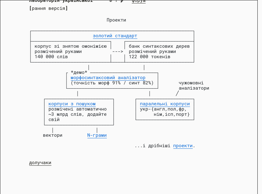
- I need to know more theory to understand but feels EXTREMELY useful
- has an API:
> curl -F json=false -F data='привіт мене звати Сірьожа' -F tokenizer= -F tagger= -F parser= https://api.mova.institute/udpipe/process
- лабораторія української
- Генеральний регіонально анотований корпус української мови (ГРАК): ГРАК - site.name
- Українська морфеміка — Вікіпедія
- Corpora UA
- brown-uk/corpus: Браунський корпус української мови
- золотий стандарт / UniversalDependencies/UD_Ukrainian-IU at dev
- Інші корпуси української мови та слов’янських мов - site.name, with info about whether it can be downloaded
- saganoren/ukr-twi-corpus: A corpus of Ukrainian Twitter texts + instructions for downloading and filtering texts.
- Linguistic Resources for the Ukrainian language on-line - Universität Regensburg
-
General evaluation bits:
-
Random UA:
- GRAC, can’t download but can use it for research
Benchmarks - generic
- Here:230928-1735 Other LM Benchmarks notes
- “literature”:
- Criterias of established benchmarks: BIG-bench/docs/doc.md at main · google/BIG-bench
- Related work of <
@ruisLargeLanguageModels2022(2022) z/d/>
Cool places with potential
- Ask Про сайт | Горох — українські словники if they can make dumps available, I could do something like “find the closest synonym to this word” etc.
- OH NICE: Home · LinguisticAndInformationSystems/mphdict Wiki
- These seem to be the DBs of the dictionaries: mphdict/src/data at master · LinguisticAndInformationSystems/mphdict
- OH NICE: Home · LinguisticAndInformationSystems/mphdict Wiki
- Cited in WSD task3:
- Open data places:
Plan, more or less
- Methodically look through and understand existing benchmarks and tasks
- Kinds of tasks
- How is the code for them actually written, wrt API and extensibility
- Do this for English, russian, Ukrainian
- At the same time:
- Start creating small interesting tasks 230928-1630 Ideas for Ukrainian LM eval tasks
- Start writing the needed code
- Write the actual Masterarbeit along the way, while it’s still easy
Changelog
- 2023-10-03 00:22: EvalUAtion is a really cool name! Ungoogleable though
-
Reproducing ARC Evals’ recent report on language model agents — LessWrong ↩︎
-
<
@labaContextualEmbeddingsUkrainian2023Contextual Embeddings for Ukrainian (2023) z/d/> / Contextual Embeddings for Ukrainian: A Large Language Model Approach to Word Sense Disambiguation - ACL Anthology ↩︎
-
Day 1722 (19 Sep 2023)
seaborn label bars in histogram plot
The ’new’ function in matplotlib for this is matplotlib.pyplot.bar_label — Matplotlib 3.8.0 documentation (ty Revisions to Display count on top of seaborn barplot [duplicate] - Stack Overflow):
ax = sns.histplot(df.langs_parsed)
#ax.set_xlabel("Language(s)")
#ax.set_ylabel("# of files")

for i in ax.axes.containers:
    ax.bar_label(
        i,
    )
The second link has infos about barplot, catplot, and countplot too!
If the text goes over the limit and the light-gray background of seaborn’s theme or something, increase the limit as:
ylim = ax.axes.get_ylim()[1]
new_ylim = ylim + 300

ax.axes.set_ylim(0, new_ylim)

# you can also set padding of the labels in px and Text (https://matplotlib.org/stable/api/text_api.html#matplotlib.text.Text) properties:
for ax in g.axes.containers:
    g.bar_label(ax, padding=-10,fontsize=5)
Disabling scientific notation / setting format
EDIT 2023-10-06: To disable scientific notation, one can use the
fmt=argument (seebar_labeldocu) where one can pass a format, including as f-string:for i in ax.axes.containers: ans = ax.bar_label( i, fmt="{:,.2f}", )There’s also a parameter that decides at which point to start to use sci. notation, I think I closed the tab with the link though+
-
Day 1717 (14 Sep 2023)
German NLP resources
It includes a really cool list of corpora!
And at the end has a list of other such pages for other languages etc.
Also: deutschland · PyPI: “A python package that gives you easy access to the most valuable datasets of Germany.”
-
Day 1714 (11 Sep 2023)
Latex print or not the entire bibliography from a file
The LREC Author’s Kit prints all things in the .bib file and it uses
\nocite{*}for that.The Internet from 2009 agreess that’s the way to go : Biblatex - Printing all entries in .bib file (cited and not)
Removing this line removes the printout.
Lastly, the link above shows printing separate bibliographies; the LREC Author’s kit does something different for the same:
\subsection{Language Resource References}

Language resource references should be listed in alphabetical order at the end of the paper.

\nocite{*}
\section{Bibliographical References}\label{sec:reference}

\bibliographystyle{lrec-coling2024-natbib}
\bibliography{lrec-coling2024-example}

\section{Language Resource References}
\label{lr:ref}
\bibliographystylelanguageresource{lrec-coling2024-natbib}
\bibliographylanguageresource{languageresource}